TL;DR

LLM Decomposition
Think about the residual stream as the highway that directly carries the contributions of every attention head and MLP ("component") to the output logits (Elhage et al., 2021). We can use these direct contributions to calculate the individual ICL accuracy of each component.
Under this view, we can (1) characterize components and (2) scale their contributions to the model output to improve few-shot accuracy.
We derive a formula: output logits = $\sum_j g_j$, where $g_j$ is the direct contribution of the component indexed by $j$. Specifically, $g_j = U \cdot C_j$, where $U$ is the output embedding matrix and $C_j$ is the post-layernorm activations of component $j$. The operation $C_j \mapsto U \cdot C_j$ is called early decoding.
*Please see §2.2 for the mathematical walkthrough, including the decomposition of the layernorm.
With the decomposition formula, we can obtain the predictions of component $j$ with ${\arg\max}_{y\in Y}\; g_j$, where $Y$ is the set of possible label words of a task, and then calculate its ICL accuracy.
*While the formula is applicable to every token, we only apply it at the last token of the input, i.e., when the model starts to generate, because we focus on classification tasks with single-token label words. We invite future work to explore generation tasks that require decomposing multiple tokens.
LLMs studied in this paper: Llama-2-7B, Llama-2-13B, Mistral-7B-Instruct-v0.1, Llama-3-8B.
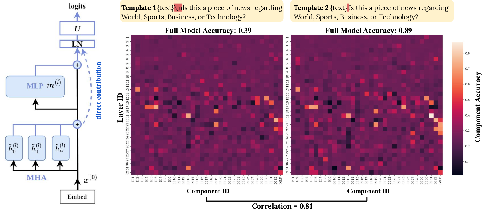
Left: Transformer decomposition. Right: We can calculate the individual accuracy of every component after decomposition. Observations: (1) Although a pair of templates that only differ slightly yield contrasting accuracies (0.39 vs. 0.89 on AGNews with Llama-2-7B), the accuracies of their internal components are highly correlated. (2) Some internal components perform much better ($+30\%$) than the full model under Template 1!
Characterizing Components
We observe three types of curious components across 8 classification tasks:
Transferability of Components
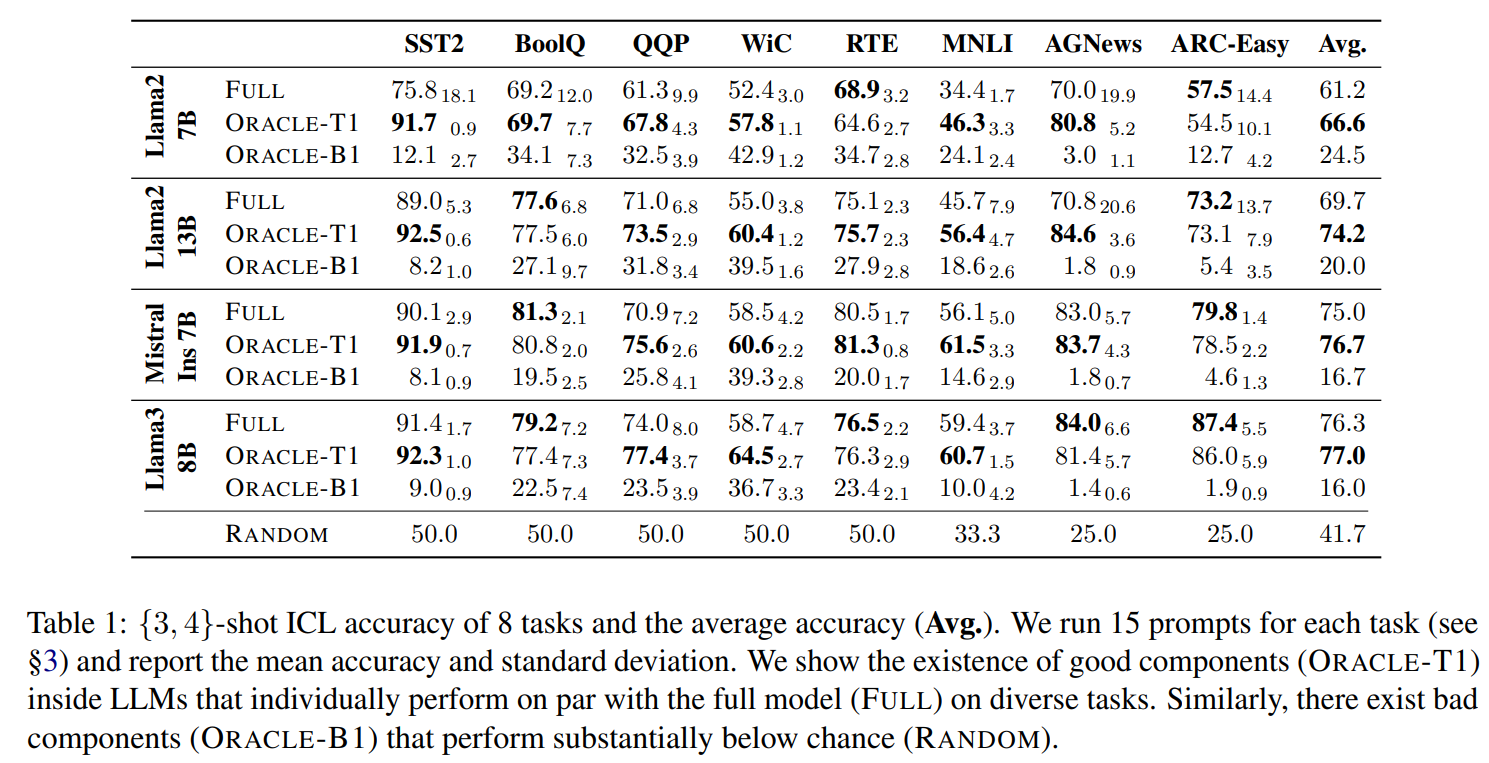
We find moderate to high component transferability across demonstrations, minimally contrastive templates, and data distributions, whereas there is much weaker transferability across randomly sampled templates. Our decomposition also uncovers the hidden abilities of individual components when the full model performs poorly.

Table 2. Given a pair of prompts (with different demonstrations or templates), we can get two lists of component accuracies and measure their agreement. We use the metrics below:
Table 3. We also evaluate whether the top-1 component selected on the source data is transferable to out-of-distribution (OOD) test data. We consider the following datasets:
Method: Component Reweighting
Our findings above show the promising direction of selecting internal components to improve ICL. Therefore, we propose a method that reweighs components by learning a weight $w_j \in \textbf{R}$ on every component, logits = $\sum_j w_j \; g_j$, where $w_j$ is initialized as $1$ for all components to match the original pretrained model.
Given $K$ (=$12$ or $24$) labeled examples, instead of using all of them as ICL demonstrations, we divide them into a demonstration set $D_{demo}$ and a training set $D_{train}$. We randomly sample $K^\prime=\{3,4\}$ examples with balanced labels as demonstrations and use the remaining examples as $D_{train}$.
We train the component weights $\{w_j\}_{j=1}^N$ with the normal cross-entropy loss for classification tasks and add an $L_1$ loss to encourage sparsity in weights.
Efficiency. Training: after extracting the component activations, we can discard the entire LLM and train a linear layer on the cached activations, which takes less than a minute on one CPU.
Inference: our method has little overhead over the standard $4$-shot ICL; much faster than the standard $K=\{12, 24\}$-shot ICL.
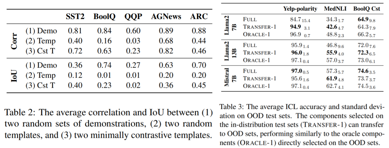
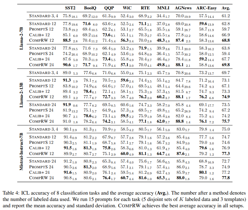
Results. Our CompRW method achieves the best average accuracy across 8 tasks:
When Do Good Components Emerge?
Do good-performing components exist in randomly initialized LLMs? No!
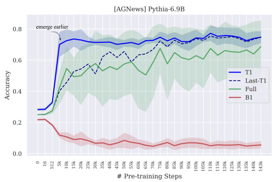
When do they emerge? Good-performing components emerge at an early stage of pretraining (blue line), while the full-model accuracy fluctuates a lot over time (green line).
$\rightarrow$ The model’s ability to do a task emerges before it is apparent from the full model.
